Effect of a Fabry–Pérot Filter on a Short Pulse: Phase, Delay, and Broadening

This tutorial continues Select One Color Between Two Mirrors: A Fabry–Pérot Narrowband Filter, using the same two DBRs, MgF₂ cavity, and transmission peak at 550 nm.

A high transmission peak tells us only how much light passes. For a short pulse, the filter also changes the phase of different frequency components, producing delay and possible pulse broadening. This tutorial reads one transmission resonance as phase, group delay (GD), and group-delay dispersion (GDD), then identifies the spectral regions most likely to change a pulse shape.

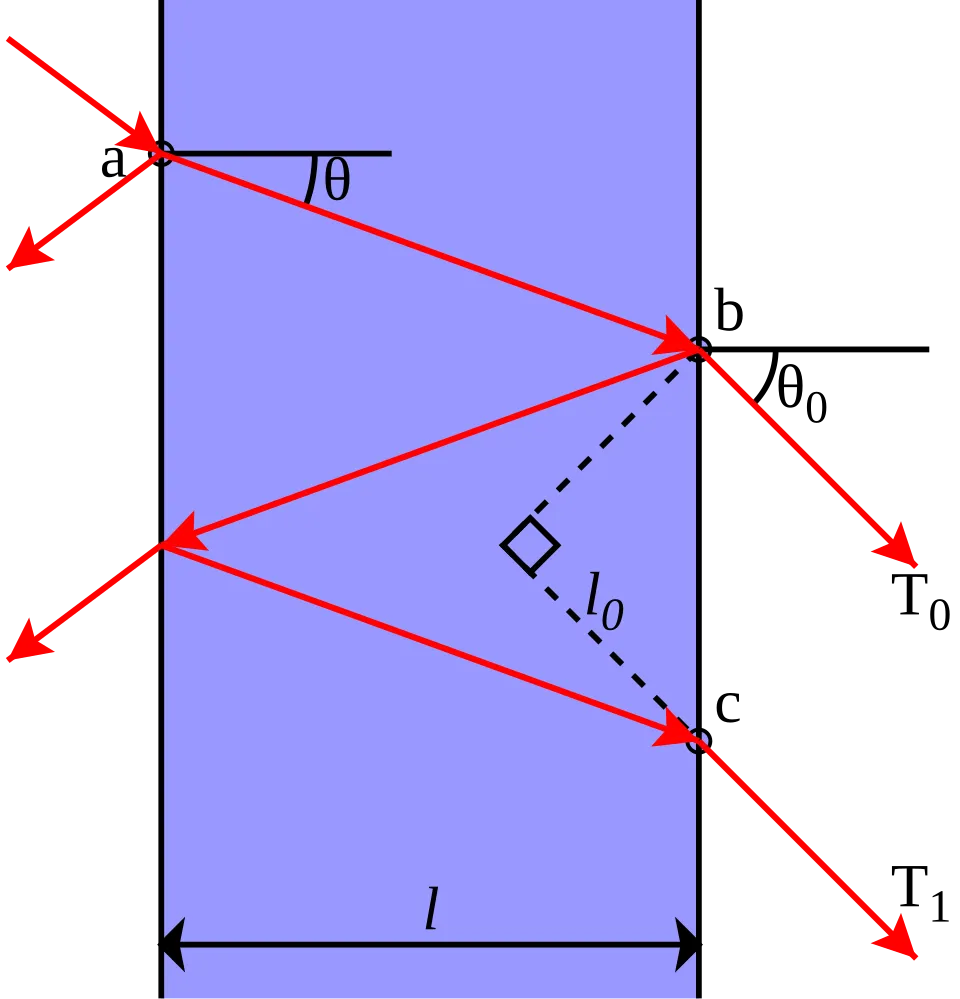
Repeated round trips between two mirrors determine both transmitted intensity and accumulated phase (Source: Krishnavedala / Wikimedia Commons · License: CC0 1.0)

From Transmittance to Phase

The complex transfer function of a filter for one frequency component can be written as

$$ H(\omega)=|H(\omega)|\exp[\mathrm{i}\phi(\omega)], \qquad E_{\mathrm{out}}(\omega)=H(\omega)E_{\mathrm{in}}(\omega). $$

Here, $\omega$ is angular frequency, $H(\omega)$ is the complex transfer function, $|H(\omega)|$ is its amplitude response, $\phi(\omega)$ is transmission phase, $\mathrm{i}$ is the imaginary unit, and $E_{\mathrm{in}}(\omega)$ and $E_{\mathrm{out}}(\omega)$ are the incident and transmitted electric-field spectra. Transmittance is determined by $|H|$; the temporal response of a short pulse also depends on how $\phi$ varies with frequency.

The first and second frequency derivatives of phase are

$$ \mathrm{GD}(\omega)=\frac{\mathrm{d}\phi}{\mathrm{d}\omega}, \qquad \mathrm{GDD}(\omega)=\frac{\mathrm{d}^{2}\phi}{\mathrm{d}\omega^{2}}. $$

GD is the delay of a narrowband pulse envelope through the filter, in fs. GDD is the rate at which GD changes with frequency, in fs². The less uniform GD is across a pulse bandwidth, the less synchronously its frequency components emerge and the greater the risk of broadening or chirp.

Reuse the 550 nm Narrowband Filter

The stack remains a front mirror, MgF₂ cavity, and back mirror. Both Layer Groups are identical to the previous tutorial, so the same structure and Edit Group configurations are reused here.

Fabry–Pérot structure reused from the previous tutorial

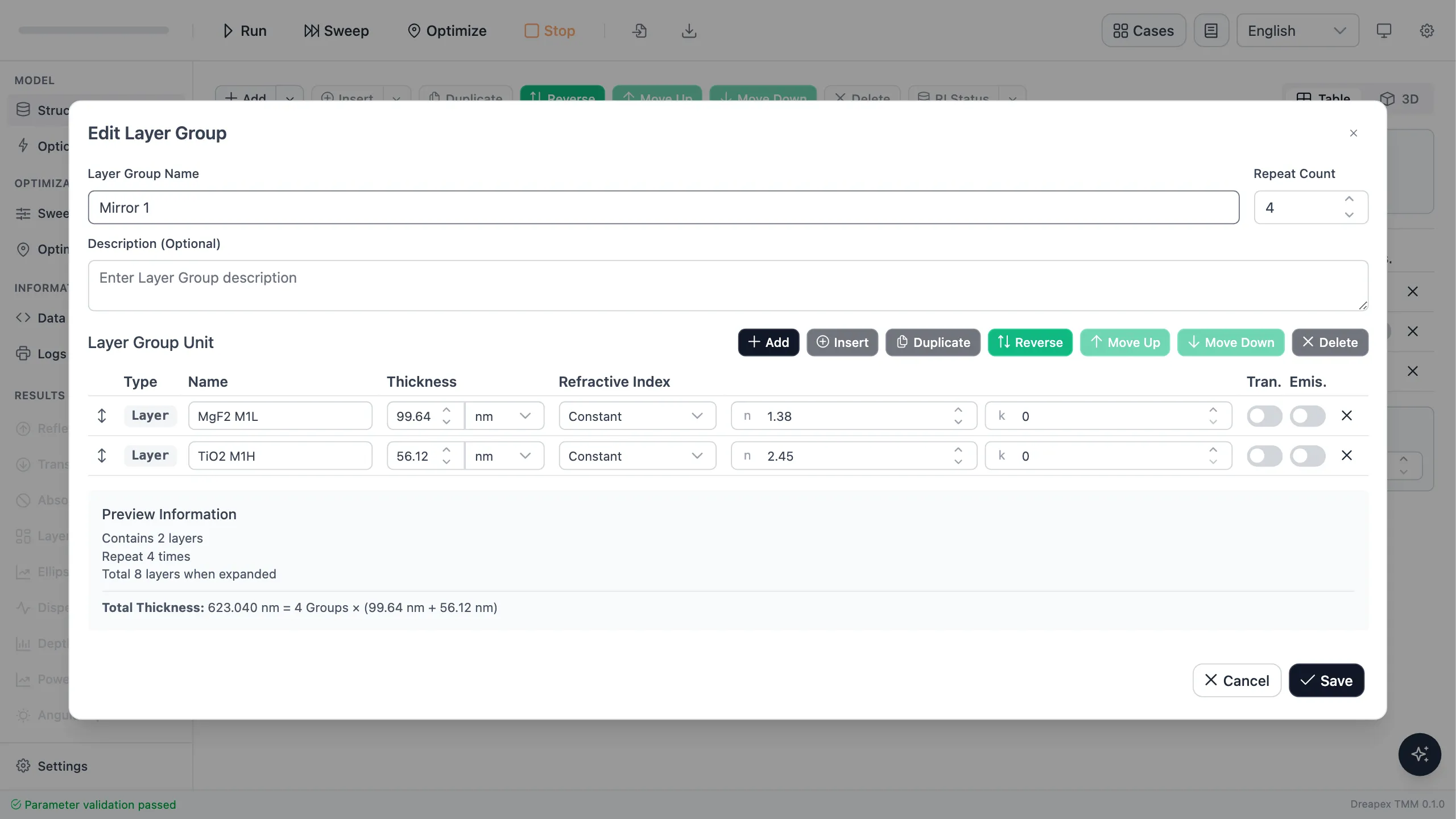
Front mirror group: MgF₂ / TiO₂ repeated four times

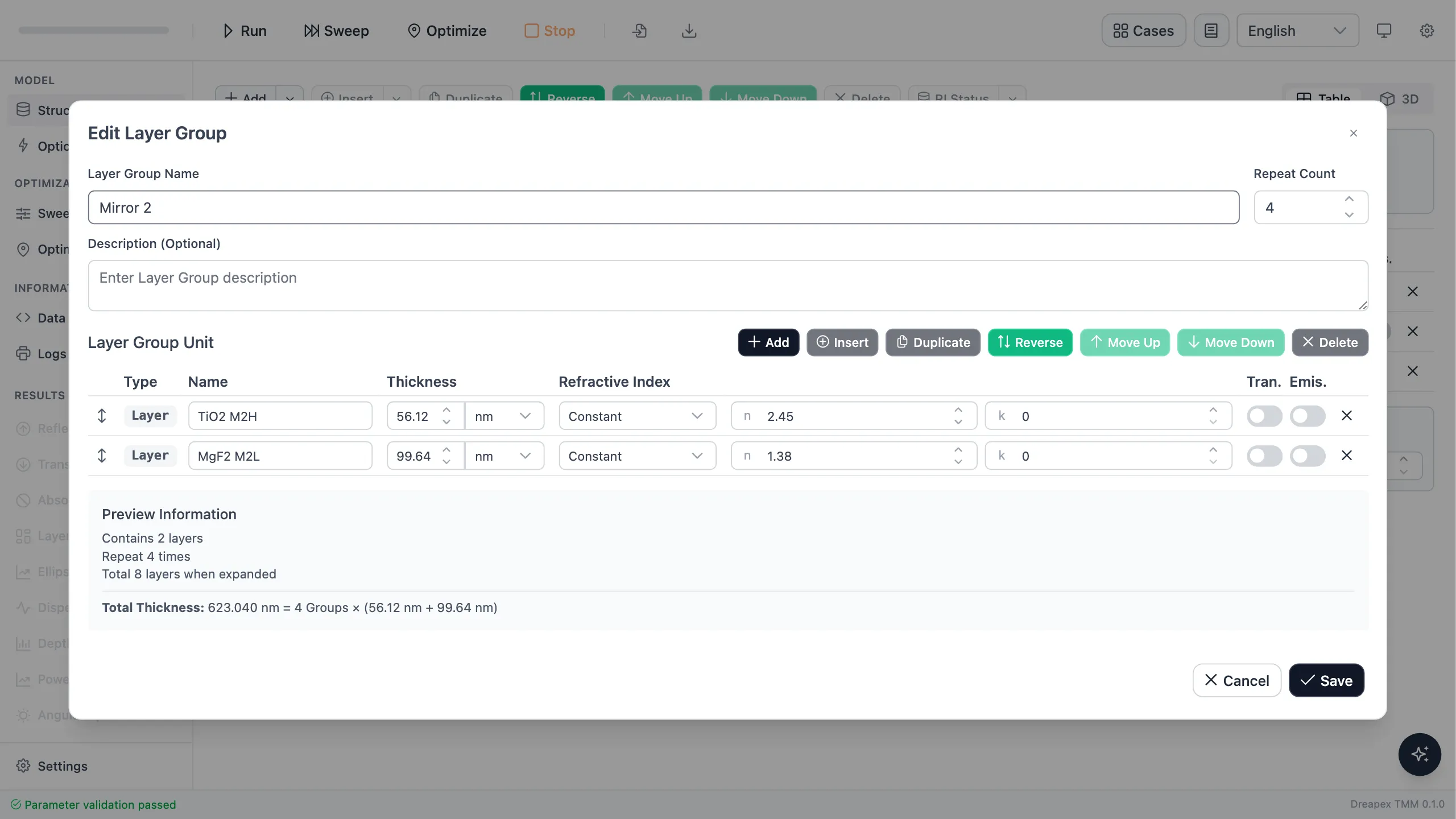
Back mirror group: TiO₂ / MgF₂ repeated four times

On the Optics page, use 540–560 nm with a 0.05 nm step, 0° incidence, and unpolarized light. Enable Transmittance, Phase, GD, and GDD. The fine step resolves the rapid phase change around the resonance.

Transmission and dispersion detectors over 540–560 nm

Locate the Transmission Peak First

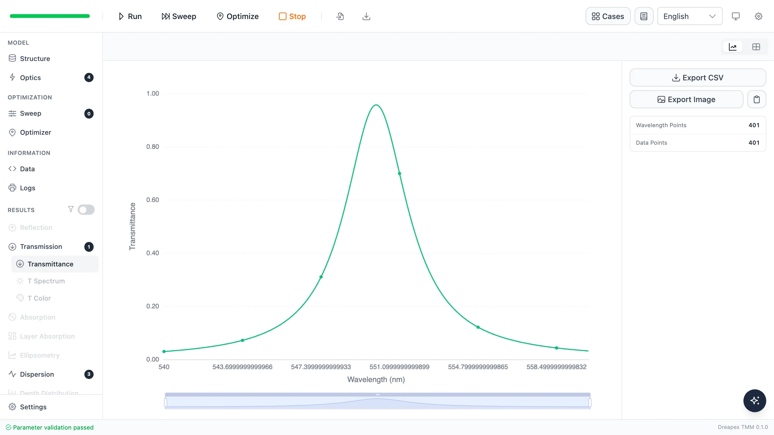
Transmission peak near 550 nm

Transmittance is 95.742% at 550 nm. At 545 and 555 nm, outside the passband, it has fallen to about 10.96% and 11.31%. If a short pulse is wider than this passband, its edge frequencies are both attenuated and subjected to a different phase response.

Phase Slope Becomes Group Delay

On the Phase result page, select Transmission and keep Unwrap Phase enabled.

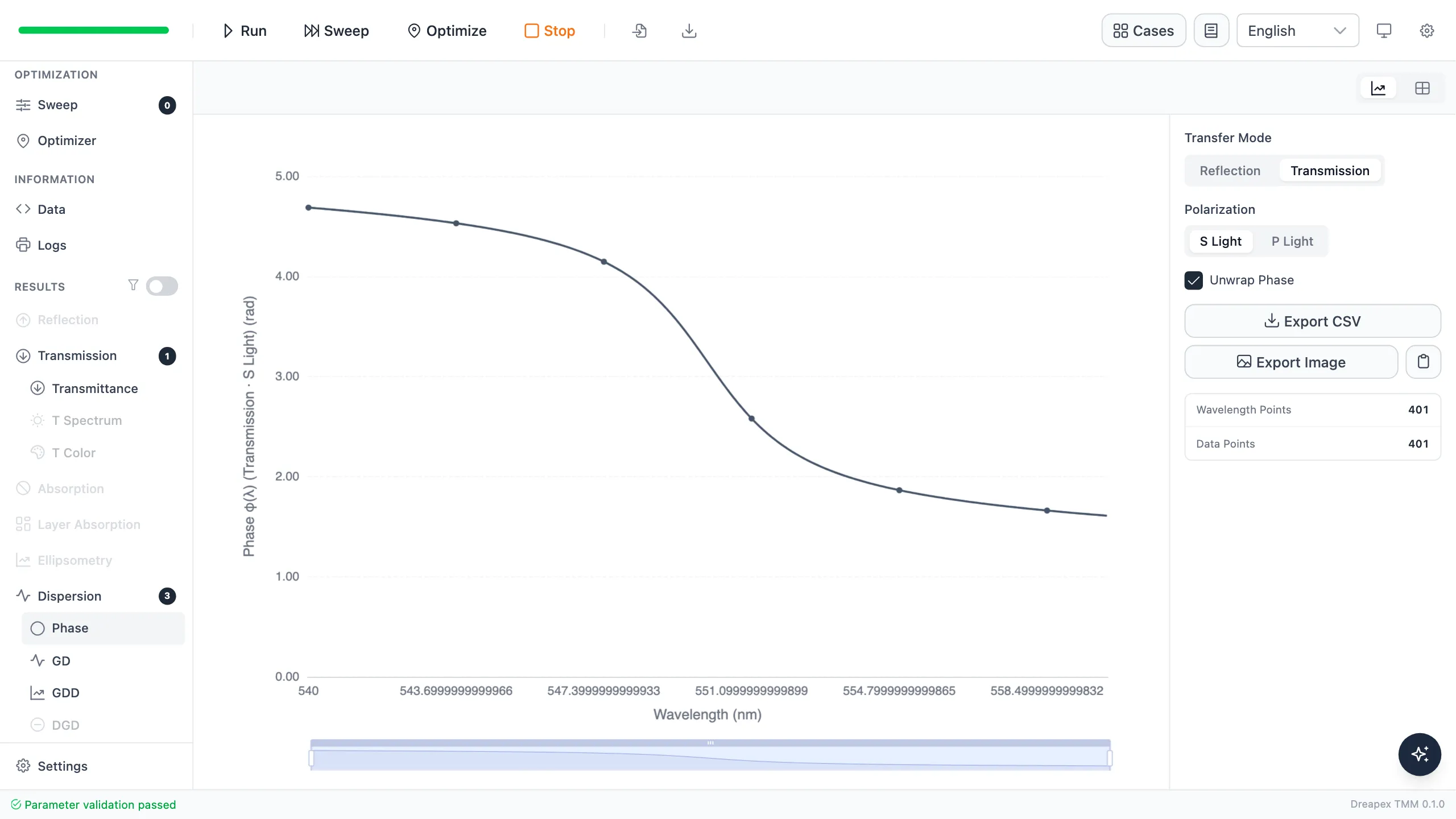
Unwrapped phase around the transmission resonance

Transmission phase changes rapidly around 550 nm. Unwrapping removes $2\pi$ jumps so the continuous slope is visible; GD is the first derivative of this curve with respect to angular frequency.

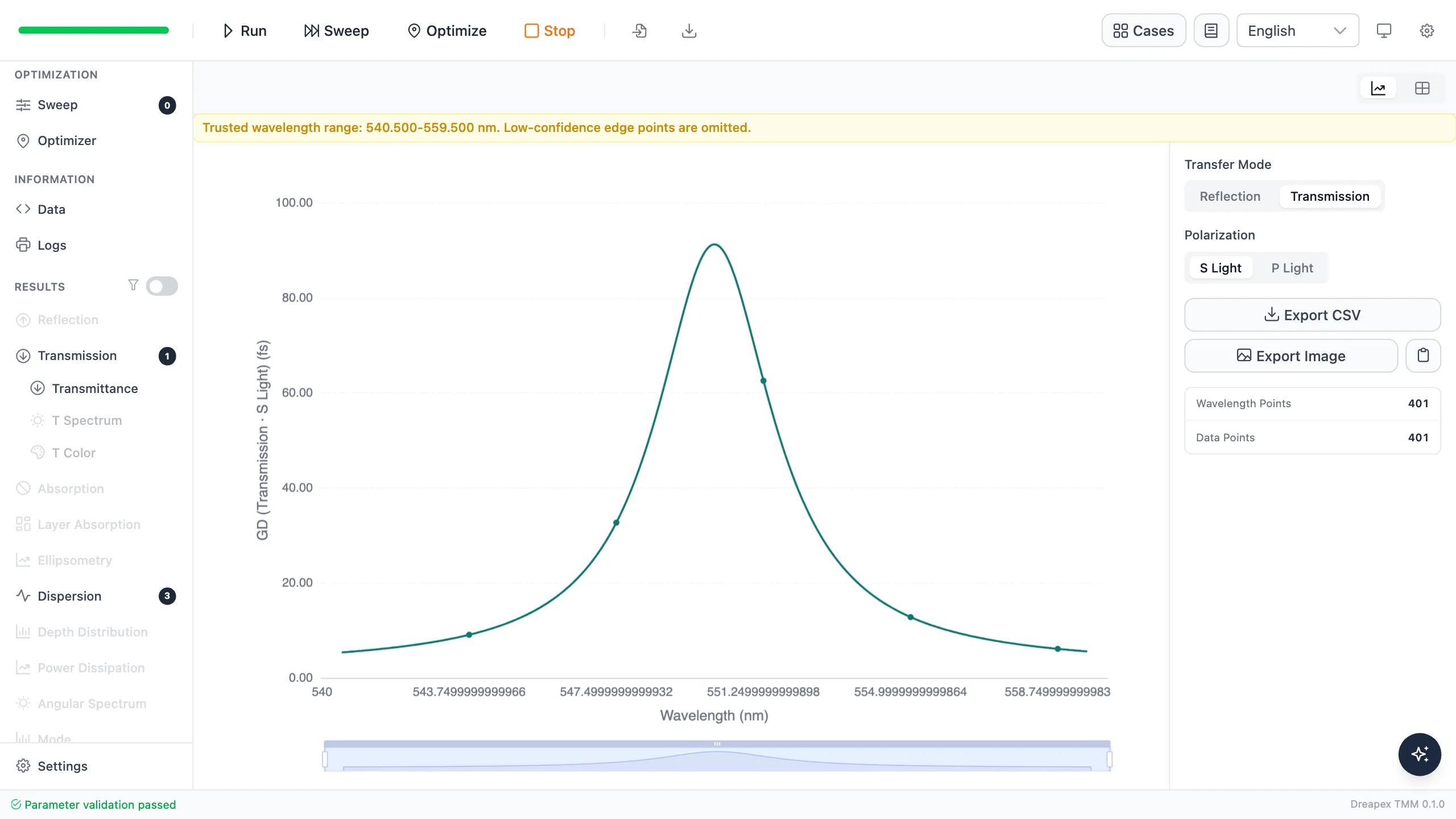
Group delay reaches its maximum at resonance

GD is about 91.23 fs at 550 nm, much larger than on either side of the passband. Physically, a resonant frequency undergoes more effective round trips in the cavity, giving the transmitted envelope a larger delay.

GDD Reveals Pulse-Broadening Risk

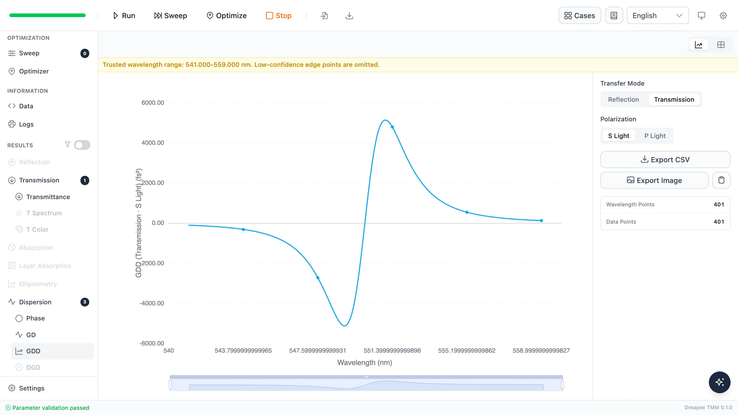
GDD has opposite signs on the two sides of the peak and crosses near its center

GDD is negative on the short-wavelength side, positive on the long-wavelength side, and crosses near 550 nm. A small band around the peak can combine high delay with low local GDD. Once a pulse spectrum spans both sides of the resonance, the strong change in GD gives different frequency components different delays.

Wavelength	Transmittance	GD	GDD
545 nm	10.96%	12.45 fs	−563.02 fs²
549 nm	73.26%	70.35 fs	−5118.96 fs²
550 nm	95.74%	91.23 fs	8.46 fs²
551 nm	73.36%	70.44 fs	5127.88 fs²
555 nm	11.31%	12.78 fs	599.55 fs²

The software differentiates discrete phase data and automatically omits low-confidence points at the wavelength limits. Interpret GD and GDD only within the trusted range shown on the result page; missing edge points do not mean that the filter has no dispersion there.

Turn Dispersion into a Design Decision

For a narrow-linewidth continuous wave, transmittance is usually the primary metric. For a short pulse, place its center wavelength and spectral bandwidth on the GD/GDD curves as well:

• At 550 nm, the filter adds about 91 fs of group delay.
• The closer and narrower the pulse spectrum is around the peak, the more uniform its GD.
• A spectrum spanning both sides of the peak encounters large GDD of opposite signs and a greater risk of broadening and chirp.
• If pulse fidelity is a design goal, constrain transmittance, GD flatness, and GDD together rather than maximizing peak transmission alone.

These results describe the filter’s frequency-domain response, not a complete time-domain pulse-propagation calculation. The output pulse duration requires the incident pulse spectrum and the complex transfer function together.

Variation Exercise

Change only the MgF₂ cavity thickness from 199.28 nm to 205 nm. Rerun T, Phase, GD, and GDD, then determine whether the transmission peak, maximum GD, and GDD zero crossing all move toward longer wavelengths.

---

← Back to Tutorial Catalog · Next: How Do Ψ and Δ Reveal Thin-Film Changes?

Going further

These tutorials cover the operating steps only. The physics behind them, the full parameter reference for each feature, how to read the results, and the algorithm validation all live on the documentation site:

• Transfer-Matrix Method — the physics and formulas behind these tutorials
• Feature Guide — complete reference for every screen and parameter
• Results — how to read each kind of output
• Open Dreapex TMM — build and simulate in the browser