Quick Start

This chapter builds a simple distributed Bragg reflector (DBR), executes a baseline calculation, and reads the first set of spectral results. By the end, you will have completed the minimum operational loop: structure modeling → optical configuration → run → result interpretation.

Scope

This chapter covers the following operating path:

1. Build a 5-period TiO2/SiO2 DBR structure in Structure.
2. Confirm illumination and detector settings in Optics.
3. Execute one standard run through the top toolbar.
4. Verify the run in Logs.
5. Inspect the reflectance stopband in the result pages.

At this stage, do not introduce incident spectra, color calculation, parameter sweeps, or optimization. Establish a stable baseline first before moving to advanced features.

Interface by Function

Before modeling, identify the four interface regions used throughout the manual.

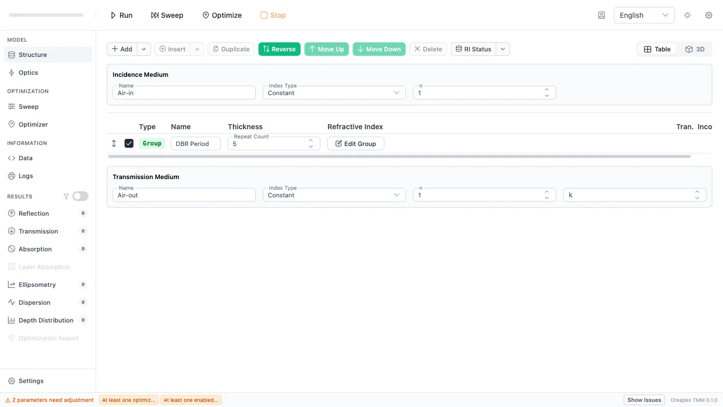
Region	Main content	Role
Top toolbar	Run, Run Sweep, Run Optimizer, Stop, documentation link (book icon), and global controls	Submit calculations, access documentation, and control execution
Left navigation	Model, Optimization, Information, Results, Settings	Move between modeling, solving, and analysis views
Main workspace	parameter forms, charts, tables, and logs	Display the active input or output context
Footer	validation state, grouped errors, and readiness feedback	Provide status and diagnostic information before and after a run

Use the left navigation to switch pages, the top toolbar to start calculations, the central workspace for input and output, and the footer to check validation and diagnostics. The book icon in the toolbar opens this documentation site directly.

Build the DBR Structure

This chapter uses a 5-period TiO2/SiO2 quarter-wave stack as the baseline model. This structure produces a distinct high-reflectance stopband in the visible range, making it an effective first simulation exercise.

Target structure: Air / (TiO2 / SiO2) × 5 / Air

Set the Surrounding Media

1. Open the Structure page.
2. Confirm that Incidence Medium is set to Air-in (constant refractive index n = 1).
3. Confirm that Transmission Medium is set to Air-out.

Clear Default Layers and Create a Layer Group

1. Select and delete the default layers in the structure table until the table is empty.
2. Click the dropdown arrow next to Add in the toolbar, then select Layer Group.
3. Name the Layer Group DBR Period and set the repeat count to 5.

Configure the Layer Group Sub-layers

Click Edit Layer Group in the DBR Period row to open the editing dialog:

1. Name the first sub-layer TiO2, set its thickness to 58 nm, and select File as the refractive-index model.
2. Use the RI database browser to search for TiO2, select main/TiO2/nk/Devore, and confirm.
3. Add a second sub-layer, name it SiO2, set its thickness to 95 nm, and select File as the refractive-index model.
4. Use the RI database browser to search for SiO2, select main/SiO2/nk/Malitson, and confirm.
5. Close the Layer Group editing dialog.

Note

58 nm and 95 nm are approximate quarter-wave thicknesses estimated for a center wavelength of ~550 nm ($d = \lambda / 4n$). The exact values depend on the material dispersion and do not need to be precise to the nanometer.

Verify the Structure

After configuration, the structure table should look like this:

Order	Type	Name	Repeat	Sub-layers
1	Group	DBR Period	5	TiO2 (58 nm) + SiO2 (95 nm)

Surrounding media: Air-in / Air-out.

Confirm that the footer shows no validation errors before proceeding.

Confirm Optical Parameters

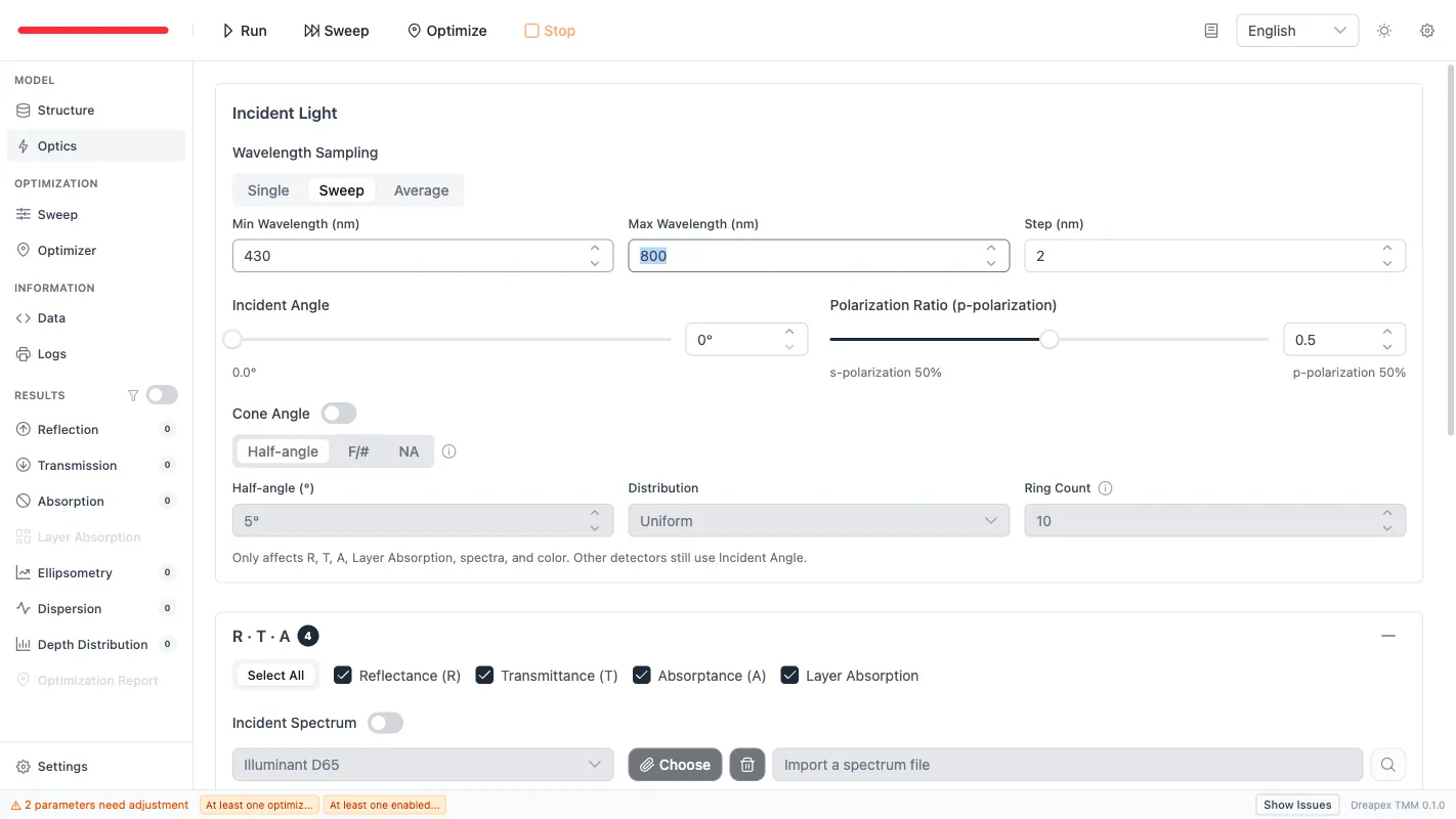
1. Open Optics.
2. Keep Incident Angle = 0°.
3. Keep pRatio = 0.5.
4. Keep the wavelength mode as Sweep.
5. Set the wavelength range: From = 430 nm, To = 800 nm, Step = 2 nm (430 nm is the lower bound of the Devore TiO2 data).
6. Confirm that R, T, A, and Layer Absorption remain enabled.
7. Keep Incident Spectrum and Visible Color disabled.

If Run is still disabled at this point, the model contains a validation error. Return to Structure or Optics, correct the invalid field, and continue only after the run control becomes available.

Execution and Run Verification

Click Run in the top toolbar.

The standard execution sequence is:

1. The application submits the current model for calculation.
2. The interface routes to Logs.
3. The log view reports whether the task has started, completed, or failed.

For the first run, verify these items in Logs before reading any result:

1. The calculation was accepted and started.
2. The calculation completed successfully.
3. No blocking error was reported.

If the task does not start, the usual cause is input validation. If the task starts but does not complete, use Logs to identify the failure and return to the model pages.

Result Interpretation

After a successful run, inspect the result pages in the following order:

1. Reflectance
2. Transmittance
3. Absorptance
4. Layer Absorption

The first three pages establish the energy balance; Layer Absorption then shows where the absorbed power is distributed inside the stack.

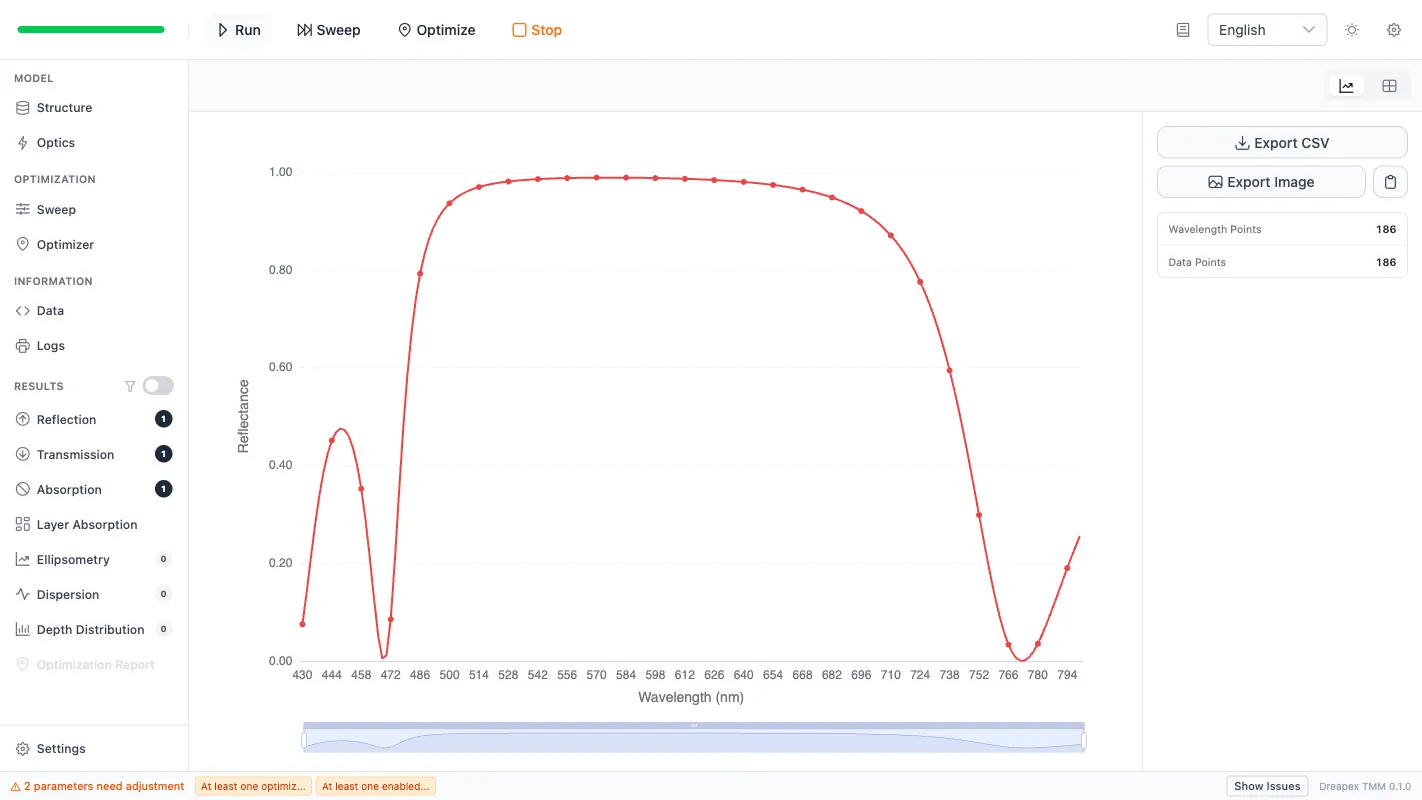
When reading the DBR reflectance result, look for the following features:

1. Stopband region: In the mid-visible range (approximately 480–740 nm), reflectance approaches 1, forming a distinct high-reflectance plateau.
2. Band edges: Reflectance drops sharply from high to low values at the band edges, forming steep transition zones.
3. Sidelobe oscillations: Equally spaced oscillation peaks appear on both sides of the stopband — this is a normal feature of a finite-period stack.
4. Energy conservation: At each wavelength, R + T + A should be close to 1. Since TiO2 and SiO2 are nearly lossless in the visible range, Absorptance should be very small.

If a result entry remains disabled, that usually means the current calculation did not generate that category of output. This is a configuration consequence, not necessarily an application error.

Baseline Validation

Use the following checks to determine whether the first calculation is physically consistent:

1. Within the stopband, Reflectance should be close to 1, and Transmittance should be close to 0.
2. On both sides of the stopband, Transmittance recovers, Reflectance drops, and sidelobe oscillations appear.
3. R + T + A ≈ 1 holds at all wavelength points.
4. In Layer Absorption, the sum of layer-resolved absorption should match the total A.

If these checks fail, inspect the following in order:

1. Whether the material selection and thickness values inside the Layer Group are correct.
2. Whether the run actually completed successfully in Logs.
3. Whether the current session restored a previous draft and the visible model no longer matches the intended baseline.

First Parameter Variation

Before moving on, perform one controlled comparison to build intuition for DBR parameter sensitivity:

1. With the current 5-period DBR, note the stopband width and peak reflectance in Reflectance.
2. Change the Layer Group repeat count from 5 to 3 and run the model again.
3. Compare the two results: with fewer periods, in-band reflectance decreases and the band edges become less steep.

This comparison isolates a single parameter (period count) and demonstrates a core DBR design rule: increasing the number of periods improves in-band reflectance and band-edge steepness.

Emission Quick Path

The DBR baseline above is a propagation simulation. For light-emitting devices such as OLEDs and QLEDs, emission simulation reuses the same structure-modeling workflow — you only add emitters and emission detectors on top of the structure:

1. Build the device layer stack (electrodes, transport layers, emissive layer) following Structure Configuration.
2. Enable the Emis. toggle for the target layer in Structure and configure at least one emitter (spectrum type, dipole orientation, position, distribution). See Emitter Setup.
3. Enable Power Dissipation, Intensity, and Mode in the Emission detector group on Optics. See Emission Detectors.
4. Click Run; propagation and emission complete in a single run.
5. Inspect the Power Dissipation, Intensity, Mode, and Emission result pages in the results sidebar.

For the full workflow and the meaning of each parameter, see Emission Modeling.

Next Steps

After you can repeat the baseline run reliably, continue in this order:

1. Read Structure Configuration to understand every structural field and editing action.
2. Read Optical Parameters to understand wavelength modes, detector groups, and source configuration.
3. Then proceed to Parameter Sweep for systematic parameter studies, or move to the result chapters for detailed interpretation.

Going further

These tutorials cover the operating steps only. The physics behind them, the full parameter reference for each feature, how to read the results, and the algorithm validation all live on the documentation site:

• Transfer-Matrix Method — the physics and formulas behind these tutorials
• Feature Guide — complete reference for every screen and parameter
• Results — how to read each kind of output
• Open Dreapex TMM — build and simulate in the browser