Microcavity PeLED Angular Emission

Author: Lezhi SUN

Microcavity top-emission perovskite light-emitting diodes Authors: Yanfeng Miao, Lu Cheng, Wei Zou, Lianghui Gu, Ju Zhang, Qiang Guo, Qiming Peng, Mengmeng Xu, Yarong He, Shuting Zhang, Yu Cao, Renzhi Li, Nana Wang, Wei Huang, and Jianpu Wang Journal: Light: Science & Applications 9, 89 (2020) · Comparison target: Figure 2a-b, Figure 2c-d · License: CC BY 4.0 https://doi.org/10.1038/s41377-020-0328-6

Miao et al. compared two devices built on the same MQW perovskite emitter. The top-emitting device sandwiches a Fabry–Pérot microcavity between a 100 nm Au bottom electrode and a 15 nm semitransparent Au top electrode; the bottom-emitting device is a conventional ITO anode with a 60 nm Au top electrode that emits through glass. The measured EQEs are 20.2% and 14.5%. Angle-resolved spectra show that the cavity concentrates emission toward the normal, while the bottom-emitting device stays Lambertian.

This case builds both published stacks in Dreapex TMM and uses Intensity to calculate angular emission from 725 to 875 nm and from 0° to 90°: the top-emitting model is compared with Figure 2a and Figure 2b, the bottom-emitting model with Figure 2c and Figure 2d. The models cover optical emission only; they do not include electrical injection, EQE, or measured radiance.

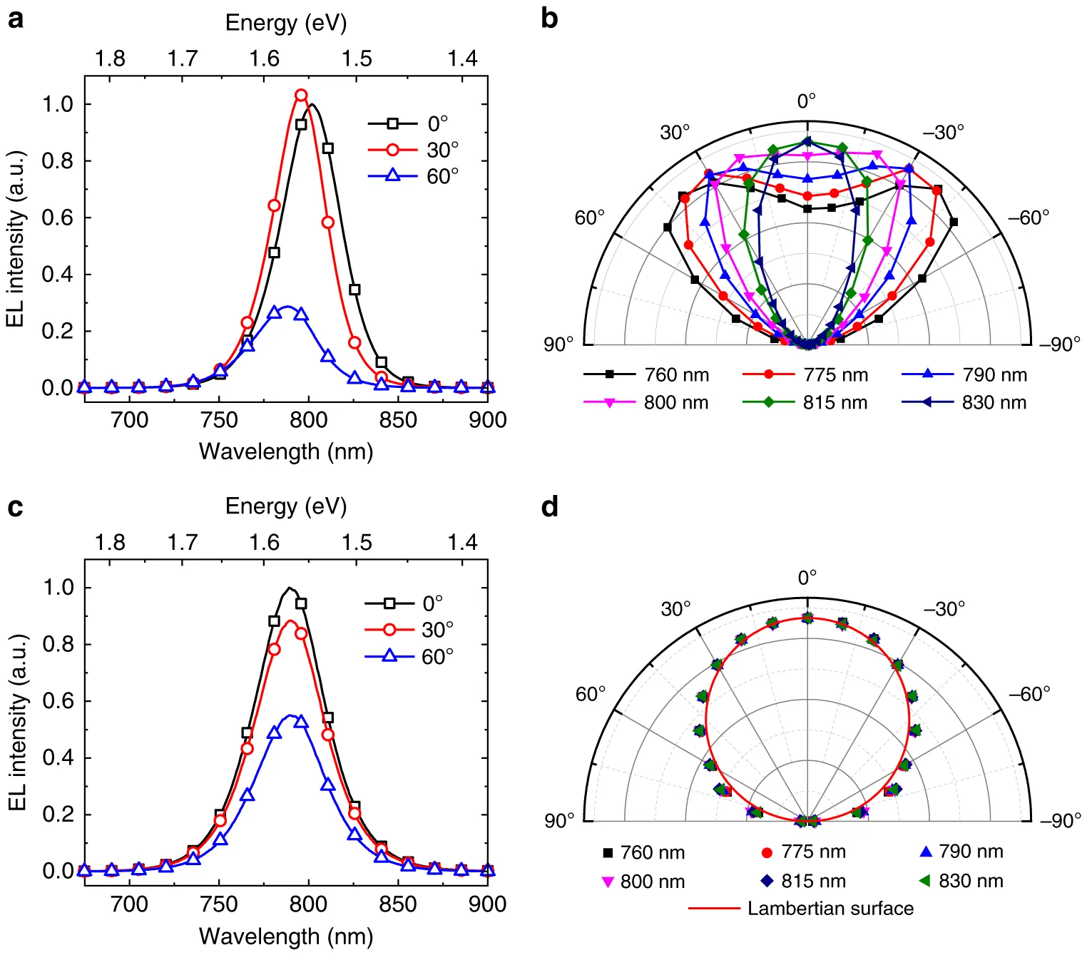
Miao Figure 2a–d, showing angle-dependent EL spectra and wavelength-resolved angular emission of the top-emitting and bottom-emitting PeLEDs. (Source: Miao et al., Light: Science & Applications (2020), Figure 2a–d · License: CC BY 4.0)

Figure 2a reports measured EL spectra at 0°, 30°, and 60°. The peak shifts to shorter wavelength with viewing angle, and the 60° peak is much weaker. Figure 2b reports angular emission at six wavelengths from 760 to 830 nm, with each curve concentrated around the surface normal. Figure 2c and Figure 2d report the same measurements for the bottom-emitting device: the peak position and linewidth do not change with viewing angle, and the angular profile follows a Lambertian distribution.

Top-emitting configuration

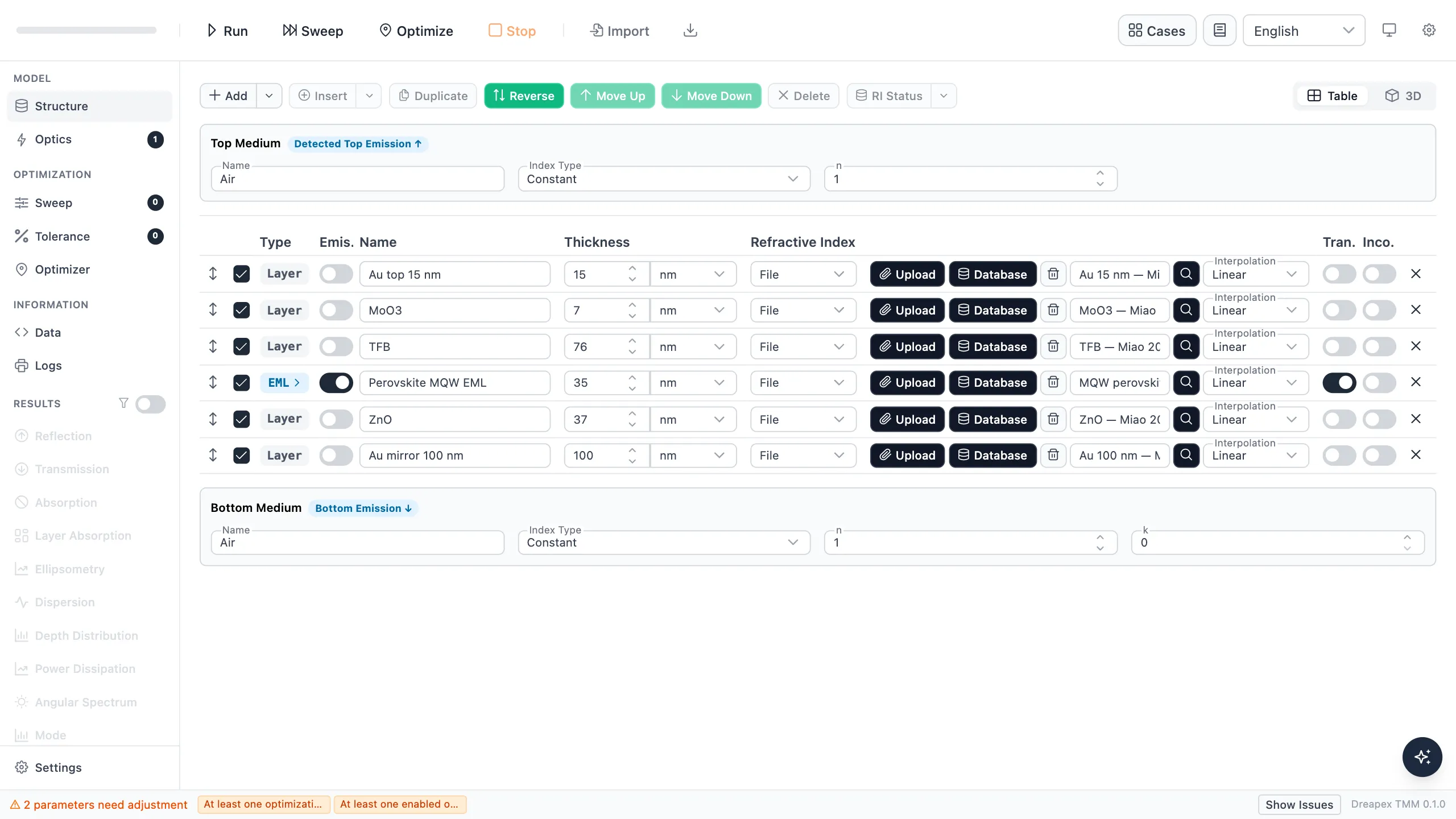
Structure configuration

The top-emitting device emits through its 15 nm semitransparent Au top electrode. Enter the layers from the emission side down to the Au mirror, in this order:

Layer	Thickness	Layer state
Au top	15 nm	—
MoO₃	7 nm	—
TFB	76 nm	—
Perovskite MQW EML	35 nm	Emis., Transparent
ZnO	37 nm	—
Au mirror	100 nm	—

The n and k values of MoO₃, TFB, MQW, ZnO, and the two Au films all come from Figure S9 of the paper’s supporting information, with the 15 nm and 100 nm Au films keeping separate datasets. The 100 nm Au mirror is nearly opaque, so the glass substrate behind it stays out of the model.

Downloadable refractive-index data

The six .nk files below were extracted from Figure S9 of the paper’s supporting information. Each file contains wavelength, refractive index $n$, and extinction coefficient $k$.

Material	Download
MQW perovskite	:case-data-download{path="/data/case-studies/microcavity-peled-angular-emission/MQW-s41377-020-0328-6.nk"}
TFB	:case-data-download{path="/data/case-studies/microcavity-peled-angular-emission/TFB-s41377-020-0328-6.nk"}
ZnO	:case-data-download{path="/data/case-studies/microcavity-peled-angular-emission/ZnO-s41377-020-0328-6.nk"}
15 nm Au film	:case-data-download{path="/data/case-studies/microcavity-peled-angular-emission/Au-15nm-s41377-020-0328-6.nk"}
100 nm Au film	:case-data-download{path="/data/case-studies/microcavity-peled-angular-emission/Au-100nm-s41377-020-0328-6.nk"}
MoO₃	:case-data-download{path="/data/case-studies/microcavity-peled-angular-emission/MoO3-s41377-020-0328-6.nk"}

Caution

The MQW file preserves the published $k$ data. After importing it into the emissive layer, enable Transparent. The emission calculation then treats this layer as $k=0$ while retaining its refractive-index dispersion.

Once the stack is entered, the Structure page shows the 15/7/76/35/37/100 nm sequence together with the EML and Transparent switches on the emissive layer:

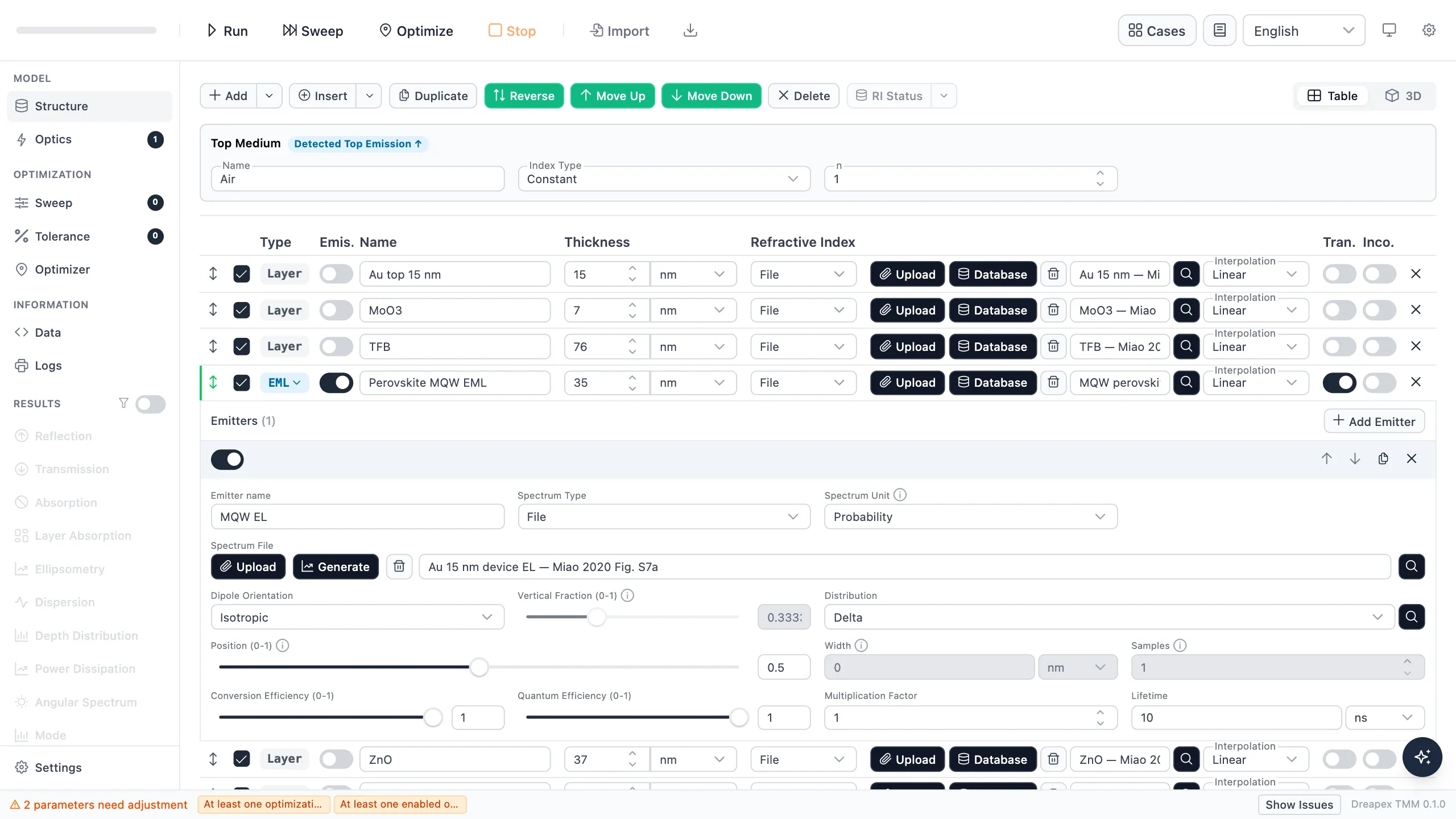
Emitter configuration table

In the MQW Emitter settings, import the :case-data-download{path="/data/case-studies/microcavity-peled-angular-emission/EL-spectrum-Au-15nm-s41377-020-0328-6.pl" label="15 nm Au device EL spectrum"}. The refractive-index and spectrum files are provided for reproducing this case. Cite Miao et al. (2020) when using them elsewhere.

The paper does not report the dipole orientation or emission-zone profile. This case uses an isotropic emitter and represents the emission zone with a single Delta sheet at the centre of the MQW.

Parameter	Value
Emitter orientation	Isotropic, vertical fraction 0.3333
Depth distribution	Delta at relative position 0.5
Conversion efficiency / quantum efficiency	1 / 1
Spectrum unit	Probability
Source spectrum	EL spectrum of the 15 nm Au device, extracted from Figure S7a

Detector configuration table

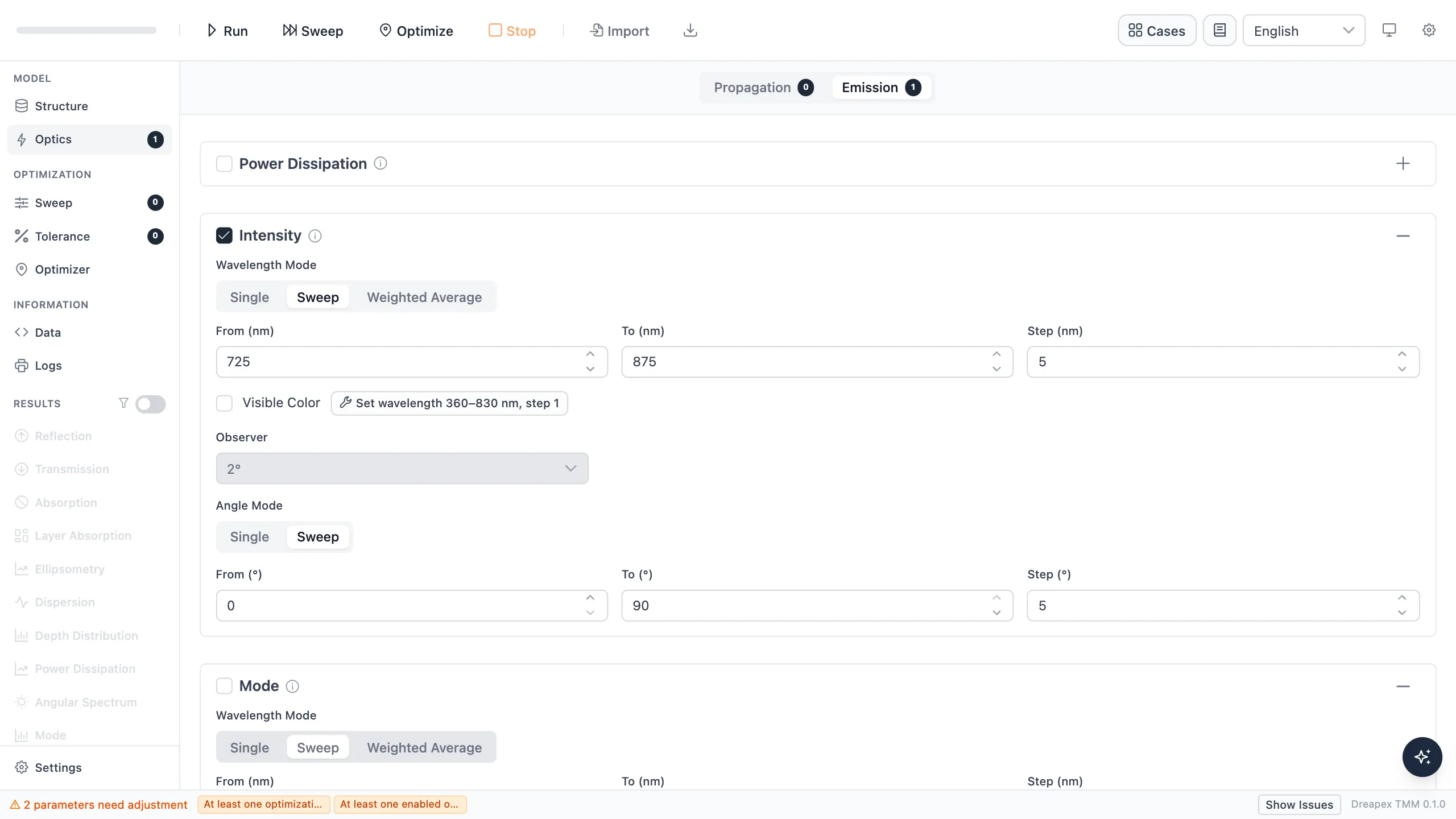
On the Emission tab in Optics, enable Intensity only and enter the wavelength and viewing-angle ranges below:

Parameter	Value
Detector	Intensity
Wavelength	725–875 nm, step 5 nm
Viewing angle	0–90°, step 5°

Note

The two notices at the bottom of the screenshot request an objective and a variable for Optimize. This case does not use Optimize, so they do not affect Run.

Top-emitting results

Figure 2a: angular spectral shift

Figure 2a retains the relative intensity difference between the three viewing angles:

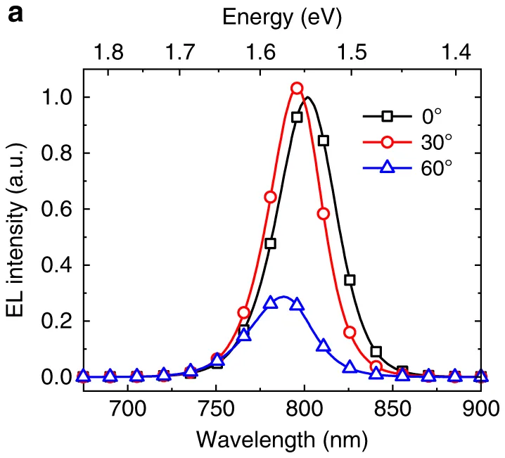
Miao Figure 2a, measured EL spectra at 0°, 30°, and 60°. (Source: Miao et al., Light: Science & Applications (2020), Figure 2a · License: CC BY 4.0)

The next screenshot comes from the same completed run. On the Intensity result page, set X-axis to Wavelength and Polarization to Total, then clear the other angles in the legend at the top right so that only 0°, 30°, and 60° stay enabled. The legend label also names the angle of each curve:

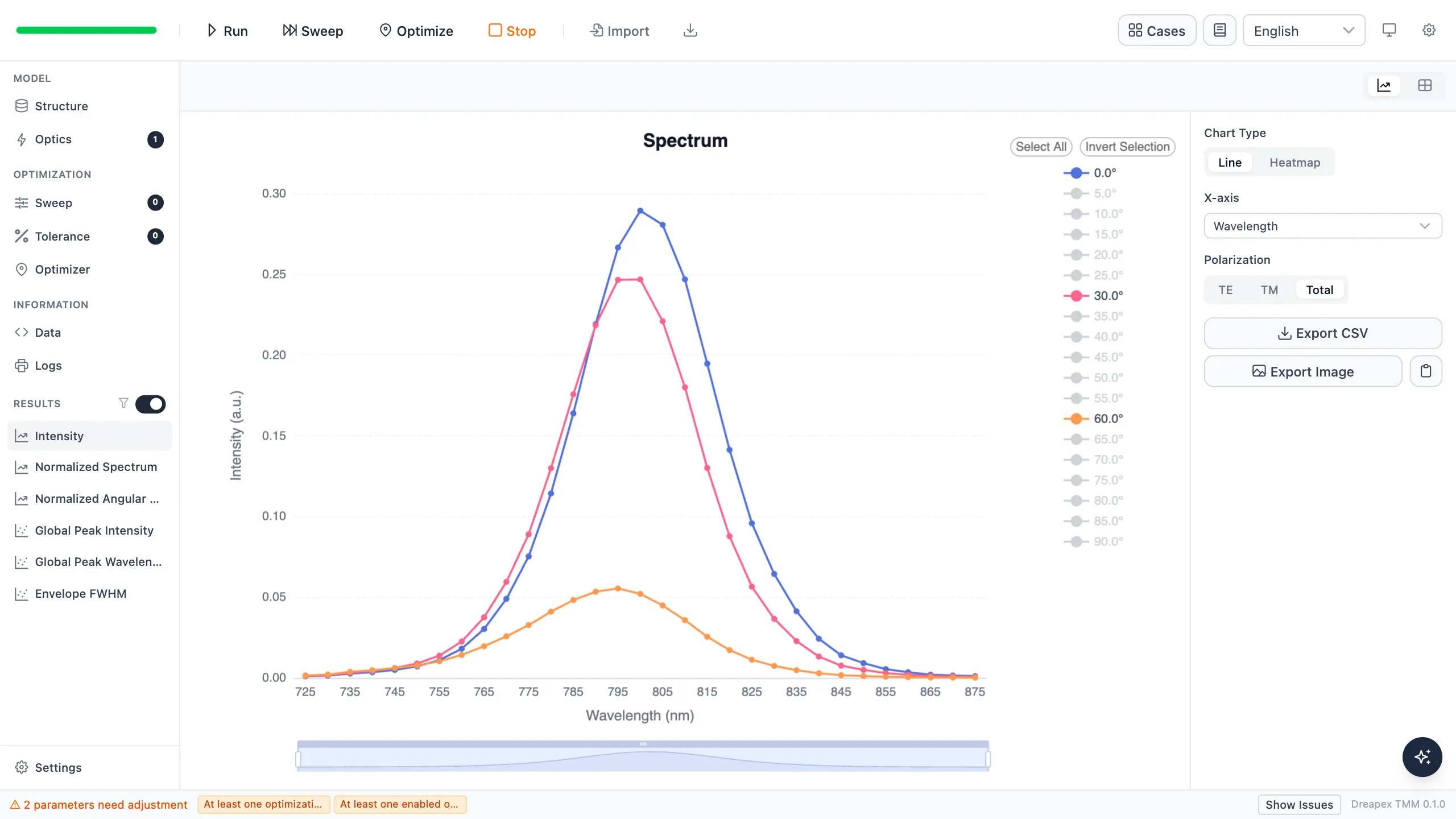
Viewing angle	Paper peak	This run, peak	Difference
0°	about 802 nm	800 nm	−2 nm
30°	about 796 nm	800 nm	+4 nm
60°	about 788 nm	795 nm	+7 nm

The calculated peak is 2 nm from the published value at 0°, 4 nm at 30°, and 7 nm at 60°. Relative to the 0° peak, the calculated peak intensities at 30° and 60° are 0.85 and 0.19. Both the intensity attenuation and the peak shift at large angles are therefore reproduced.

The wavelength accuracy of the spectral simulation is insufficient and produces an error. Reducing the wavelength-sampling Step gives a more accurate peak position. The intrinsic emission spectrum without the cavity response was not available either, so the model imports the TE-PeLED EL spectrum from Figure S7a, which introduces a further deviation.

Figure 2b: angular emission pattern

Figure 2b reports normalized angular emission at six wavelengths:

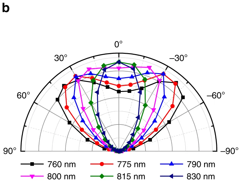
Miao Figure 2b, measured angular emission at six wavelengths. (Source: Miao et al., Light: Science & Applications (2020), Figure 2b · License: CC BY 4.0)

Switch the result to Normalized Angular Distribution, enable Polar view, and select the same six wavelengths:

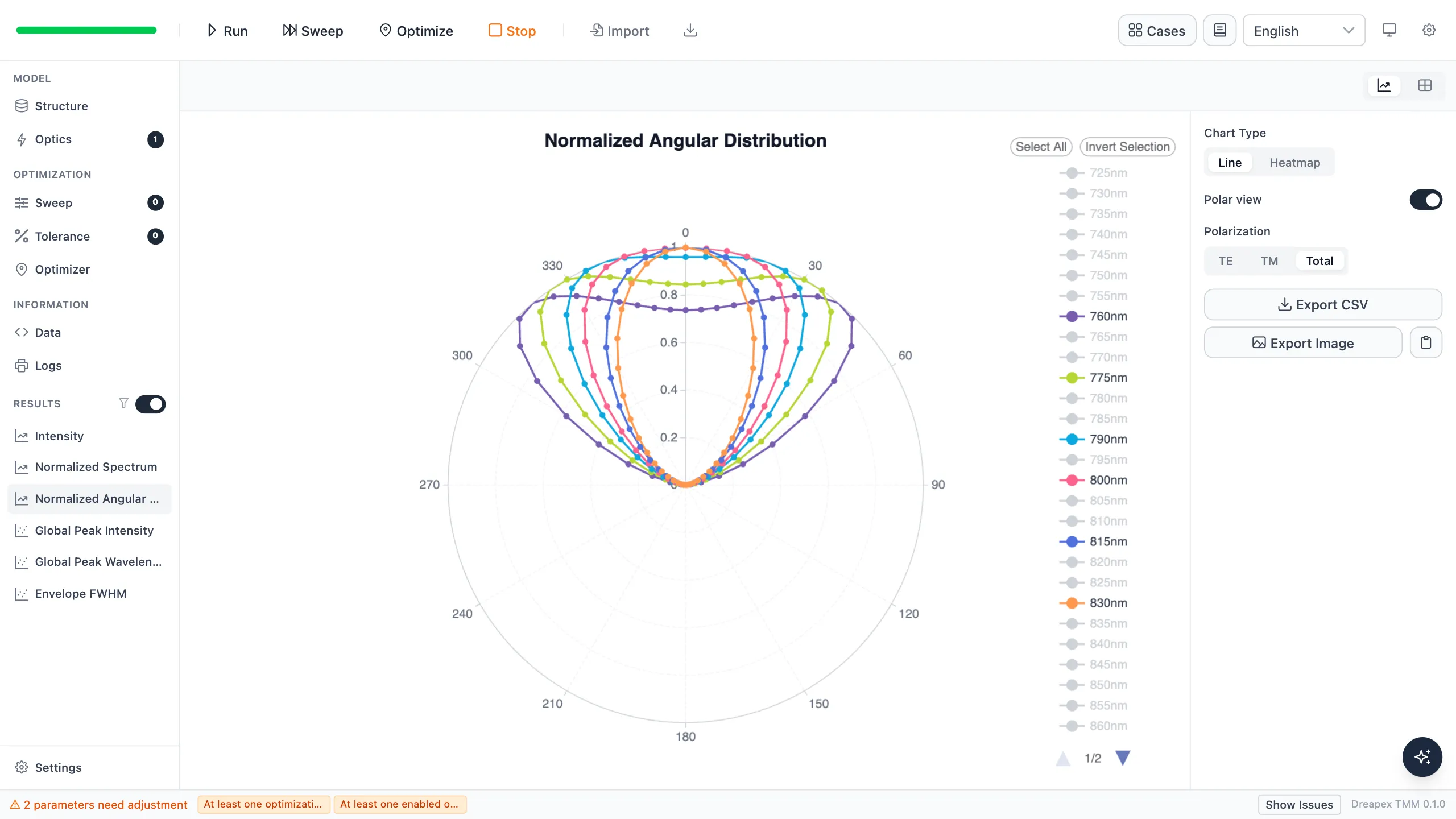
All six curves reach their maximum along the normal and narrow with increasing wavelength. The half-maximum angle decreases from about 60° at 760 nm to about 35° at 830 nm, matching the trend in Figure 2b.

Bottom-emitting configuration

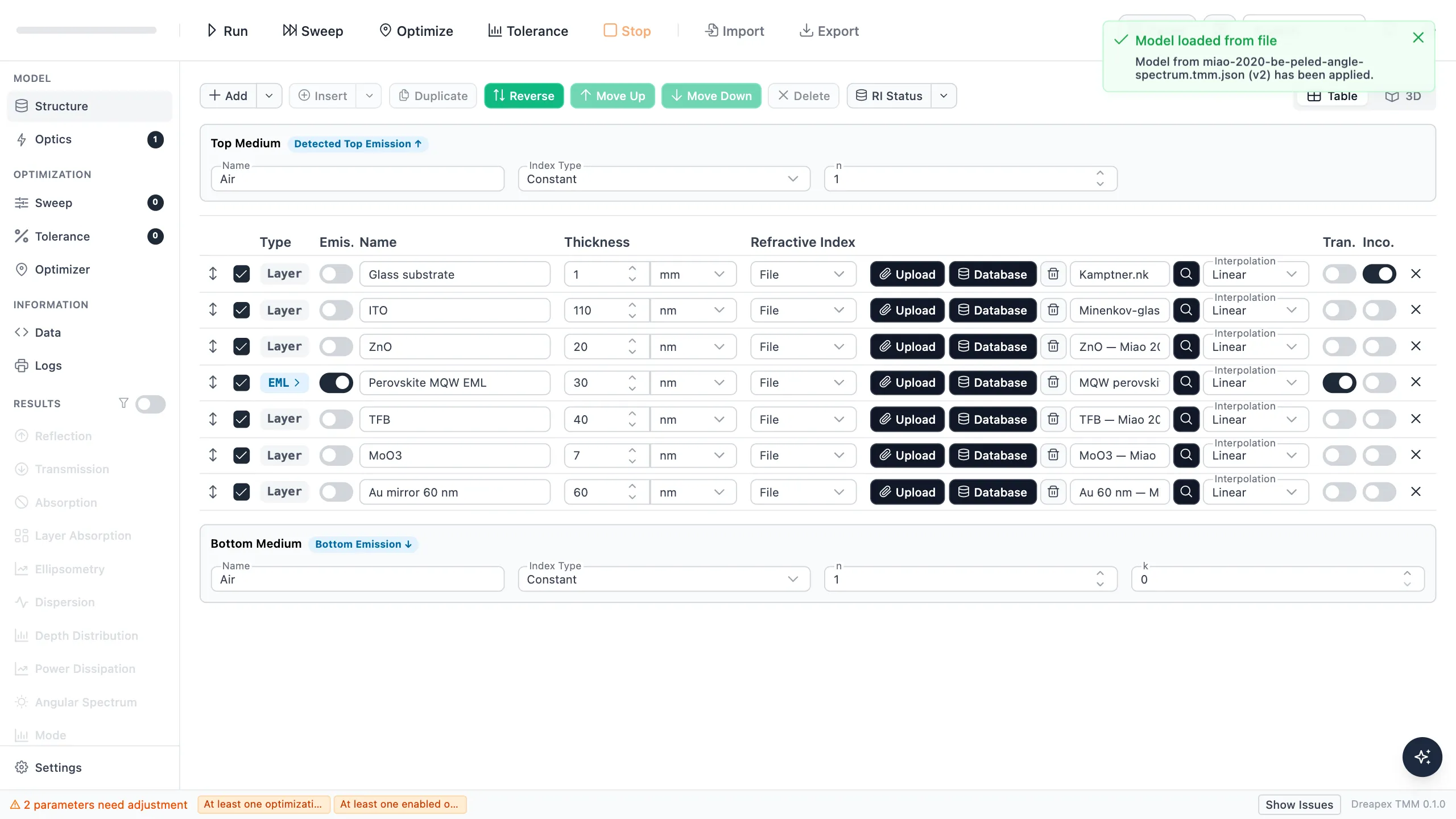
Structure configuration

The bottom-emitting device emits through its glass substrate and shares the emitter with the top-emitting device, but both contact layers have different thicknesses. Set Glass as an incoherent layer (Inco.) and the MQW layer as the emissive layer (Emis.).

Intensity reports emission toward the Top Medium side. A bottom-emitting model therefore has to place the substrate on that side: enter Glass substrate in the first Structure row, followed by ITO, ZnO, the emissive layer, the hole-transport layer, and MoO₃, with Au mirror 60 nm in the last row. In the run screenshot, Top Medium Air is adjacent to the first glass row, so light exits upward through the glass; Bottom Medium Air is on the Au side. Both surrounding media are Air.

Layer	Thickness	Layer state
Glass substrate	1 mm	Inco.
ITO	110 nm	—
ZnO	20 nm	—
Perovskite MQW EML	30 nm	Emis., Transparent
TFB	40 nm	—
MoO₃	7 nm	—
Au mirror 60 nm	60 nm	—

Figure S4 of the supporting information gives this stack, in which the electron contact is PEIE-modified ZnO on ITO; the model merges that with ZnO into a single 20 nm layer. MoO₃, TFB, MQW, and ZnO keep the Figure S9 optical constants of the top-emitting model. The paper reports ITO without optical constants or thickness, so this case uses Minenkov-glass from the refractive-index database (110 nm commercial sputtered ITO) and Kamptner soda-lime glass for the substrate.

Emitter configuration table

The bottom-emitting model reuses the top-emitting emitter settings and uses the EL spectrum of the same MQW film:

Parameter	Value
Source spectrum	EL spectrum of the 15 nm Au device (same as the top-emitting model)
Emitter orientation	Isotropic, vertical fraction 0.3333
Depth distribution	Delta at relative position 0.5
Conversion efficiency / quantum efficiency	1 / 1
Spectrum unit	Probability

The emitter is identical to Figure 3:

Detector configuration table

On the Emission tab in Optics, enable Intensity only and enter the wavelength and viewing-angle ranges below:

Parameter	Value
Detector	Intensity
Wavelength	725–875 nm, step 5 nm
Viewing angle	0–90°, step 5°

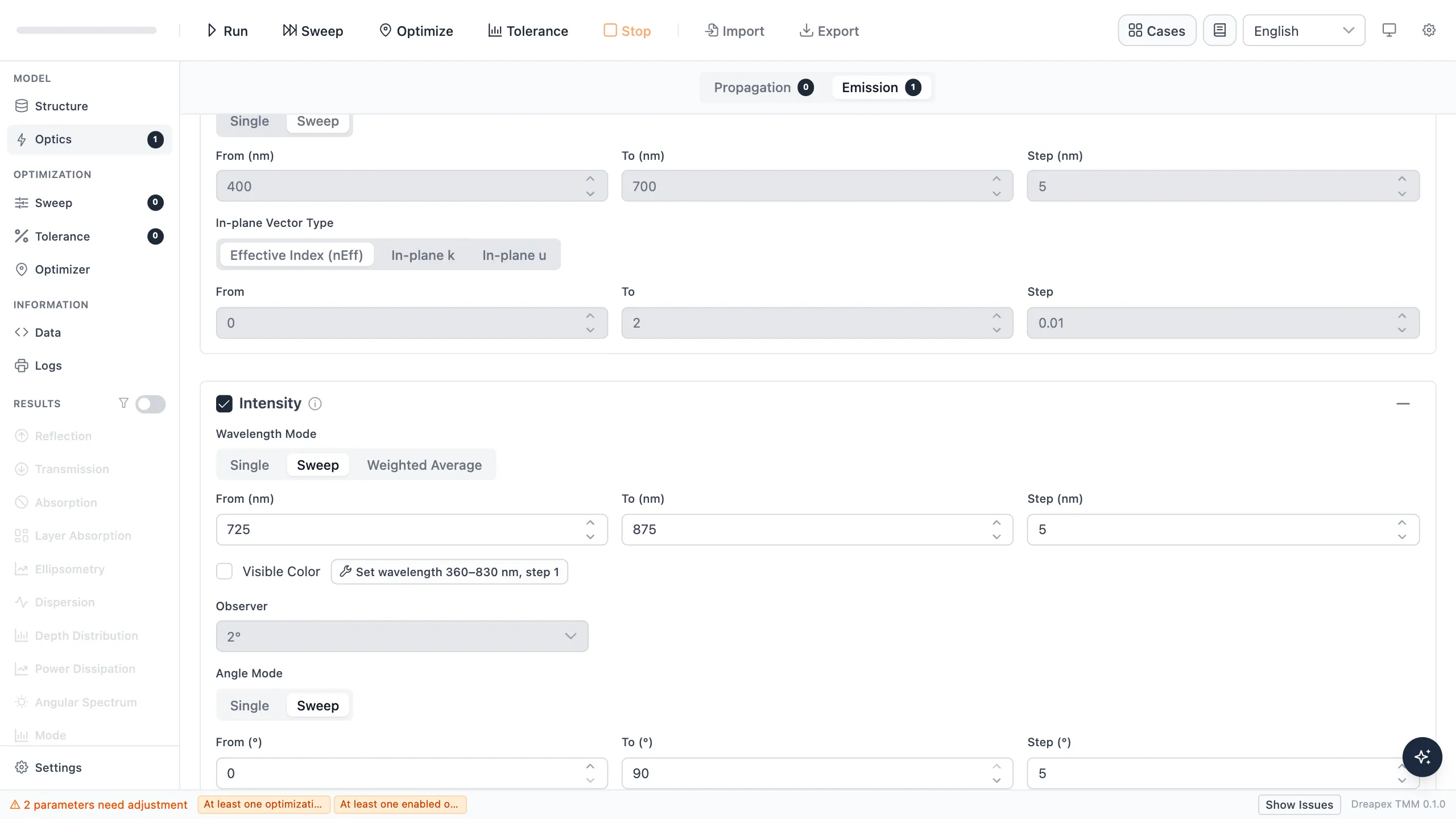
The simulated data are available as :case-data-download{path="/data/case-studies/microcavity-peled-angular-emission/BE-intensity-s41377-020-0328-6.csv" label="Dreapex TMM simulation data: bottom-emitting Intensity spectra"}, with columns for angle, wavelength, and TE / TM / Total intensity.

Bottom-emitting results

Figure 2c: bottom-emitting spectra do not move with angle

Figure 2c shows the bottom-emitting device in the same coordinates as Figure 2a:

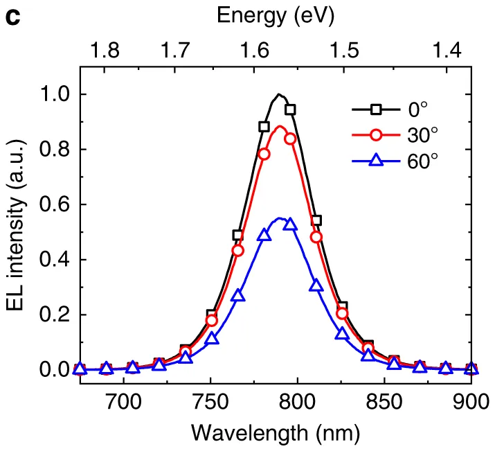
Miao Figure 2c, measured EL spectra of the bottom-emitting PeLED at 0°, 30°, and 60°. (Source: Miao et al., Light: Science & Applications (2020), Figure 2c · License: CC BY 4.0)

After the bottom-emitting run, set X-axis to Wavelength and Polarization to Total on the Intensity result page, then clear the other angles in the chart’s upper-right Legend so that only 0°, 30°, and 60° remain enabled:

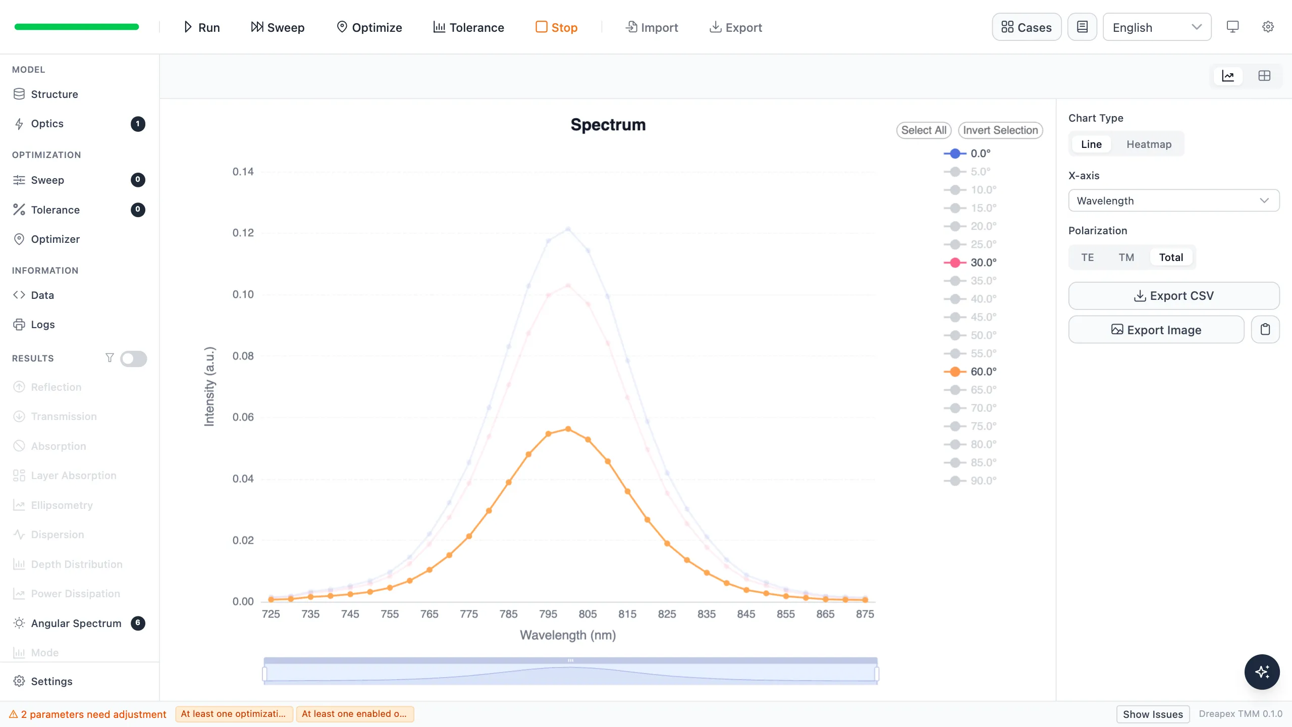
The peak values below come from the CSV exported from the same run, and the paper column is read off Figure 2c.

Viewing angle	Paper peak	This run, peak	Difference
0°	about 790 nm	800 nm	+10 nm
30°	about 790 nm	800 nm	+10 nm
60°	about 790 nm	800 nm	+10 nm

All three calculated peaks sit at 800 nm, 10 nm from the approximately 790 nm read off the published figure, and do not move with angle. The paper curves have a read-off full width at half maximum of about 44 nm, while the three sampled curves here are about 40 nm wide.

The intrinsic emission spectrum without the cavity response was not available, so the model imports the TE-PeLED EL spectrum from Figure S7a, which introduces a deviation.

Figure 2d: Lambertian angular profile of the bottom-emitting device

Figure 2d gives the angular emission at six wavelengths in polar coordinates together with a Lambertian reference:

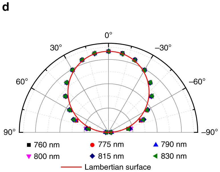
Miao Figure 2d, measured angular emission of the bottom-emitting PeLED at six wavelengths with a Lambertian reference. (Source: Miao et al., Light: Science & Applications (2020), Figure 2d · License: CC BY 4.0)

From the same run, open Normalized Angular Distribution, enable Polar view, click Invert Selection in the Legend, and select 760nm, 775nm, 790nm, 800nm, 815nm, and 830nm:

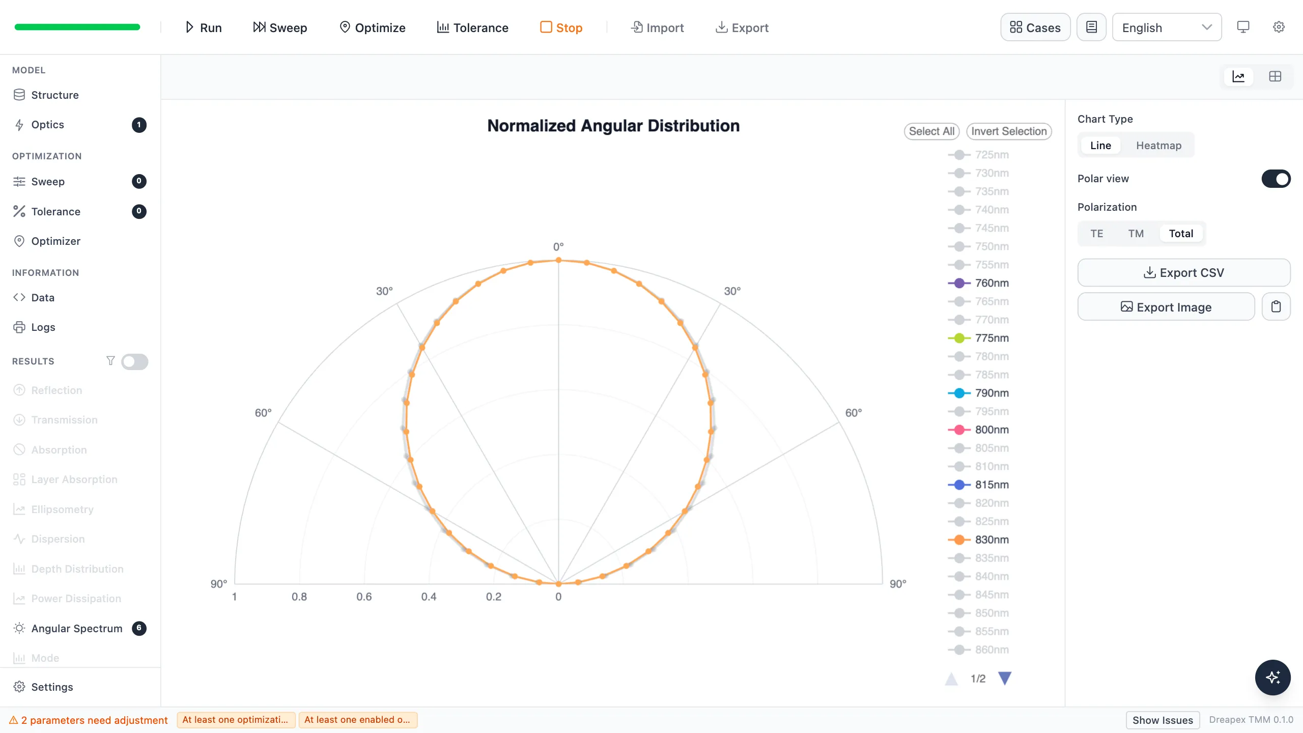
The six wavelength curves nearly overlap, all peak along the normal, and fall to half maximum near 60°. The values below are the mean of the six selected curves at each angle, normalized to their normal-direction intensity:

Viewing angle	This run	Lambertian $\cos\theta$
0°	1.000	1.000
30°	0.848	0.866
50°	0.609	0.643
60°	0.463	0.500
80°	0.144	0.174

At 30°, 50°, 60°, and 80°, the absolute differences from the Lambertian reference are about 0.02, 0.03, 0.04, and 0.03. This follows the Lambertian trend in Figure 2d.

Deviation Notes

• Smaller top-emitting angular blue shift: the calculation moves the peak by 5 nm from 0° to 60°, compared with about 14 nm in Figure 2a. The source is a measured device EL spectrum that already contains the cavity response; the ideal input is an MQW photoluminescence spectrum without it.
• ITO in the bottom-emitting model: the paper does not provide the ITO refractive index, so database data is used, which may introduce a small error.
• Substitute ITO data: Figure S9 does not include ITO. This case uses the 110 nm commercial sputtered ITO entry from the refractive-index database and takes the thickness from that sample; the substitution affects the cavity length and outcoupling of the bottom-emitting device.
• Emissive layer treated as transparent: the published MQW file has nonzero $k$ over 725–875 nm, so the model enables Transparent and the emission calculation uses $k=0$ while keeping the refractive-index dispersion.
• Sampling resolution: 5 nm wavelength steps and 5° angle steps, with about ±2 nm of peak-position uncertainty from figure reading and grid interpolation.

Back to Case Studies · Next: Top-Emitting QLED Outcoupling

Going further

These tutorials cover the operating steps only. The physics behind them, the full parameter reference for each feature, how to read the results, and the algorithm validation all live on the documentation site:

• Transfer-Matrix Method — the physics and formulas behind these tutorials
• Feature Guide — complete reference for every screen and parameter
• Results — how to read each kind of output
• Open Dreapex TMM — build and simulate in the browser